Sparse Attention Guide: What Should an LLM Ignore?
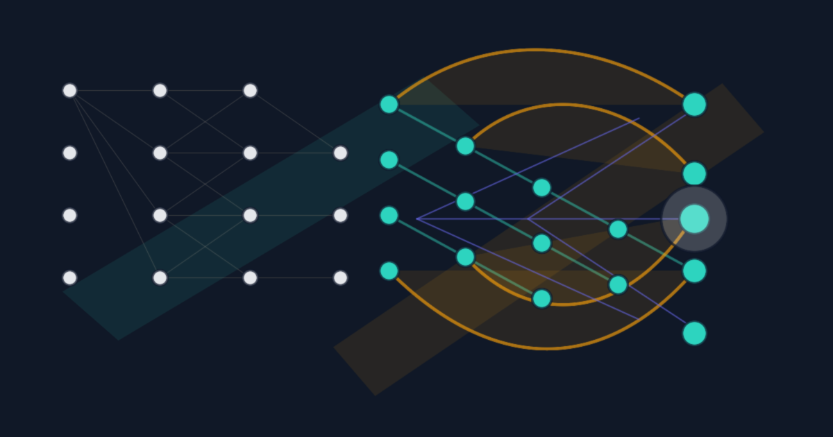
Long-context LLMs are trying to do more than remember extra text. They are trying to decide which parts of the text are still worth looking at.
That distinction matters. A model can accept 100,000 tokens, store them in memory, and still face the harder question at every layer: which previous tokens should influence the next computation? Full attention gives the cleanest answer. Every token can look at every previous token. It is powerful, simple, and expensive.
Sparse attention starts with a refusal. Maybe every token does not need to talk to every other token.
Sparse attention is a family of attention patterns where each token attends to selected tokens instead of every visible previous token.
Key Takeaways
- Full attention gives maximum visibility, but causal attention exposes roughly
n x npossible token pairs as context grows.- Sparse attention is graph design. Local, global, random, LSH, landmark, routing, and block-sparse methods keep different edges.
- Sliding windows can bound KV cache memory, but they do it by making distant tokens invisible unless another mechanism preserves them.
- FlashAttention is not sparse attention. It keeps the same connections and changes how the computation moves through GPU memory.
- Attention sinks show that attention is also geometry and stabilization, not semantic relevance alone.
Why is full attention expensive?
The original Transformer uses scaled dot-product attention, where each query compares with keys and then mixes values ( Attention Is All You Need , 2017). In a causal language model, token i can attend to tokens 1...i, so the visible token pairs grow roughly like n x n.
The mechanism is small enough to write on a napkin:
Q = Query: what am I looking for?
K = Key: what information do I offer?
V = Value: what content do I carry?

scores = Q x K^T
weights = softmax(scores)
output = weights x VFor one token, this is intuitive. The current token asks a question with Q, previous tokens advertise themselves with K, and the model blends their V vectors according to the softmax weights.
For a long sequence, the cost is the problem. If the context length doubles, the number of possible attention comparisons grows about four times. That is the shape of quadratic cost.
1,000 tokens  -> about 1,000,000 token pairs
2,000 tokens  -> about 4,000,000 token pairs
4,000 tokens -> about 16,000,000 token pairsThis is why “just make the context longer” is not a complete answer. Longer context gives the model more possible evidence, but it also creates a bigger visibility problem. At each layer, the model must decide where information should flow.
For related context on why model efficiency changes practical deployment, see the BitNet piece on 1-bit LLMs and additive inference .
How does sparse attention change the graph?
Sparse attention removes attention edges from the full graph. BigBird combines local, random, and global attention and reports a sparse mechanism that reduces the quadratic dependency to linear in its design. The important shift goes beyond asymptotic cost. It is the graph the model is allowed to build.
Think of tokens as nodes and attention connections as edges.
full attention:
every token -> every visible previous token

sparse attention:
every token -> selected previous tokensThat makes sparse attention less like a single optimization and more like a family of graph designs. Every variant answers the same question differently: who should talk to whom?
Personal note: I noticed while turning my own sparse-attention study notes into this article that the graph framing does most of the teaching. Once the reader sees tokens as nodes and attention as edges, the named variants stop feeling like jargon.
Once you see attention as a graph, the variants stop feeling like disconnected tricks.
Local attention says nearby nodes matter most. Global attention says a few nodes should coordinate the whole document. Random attention says the graph needs shortcuts. LSH attention says similar content should meet. Landmark attention says the model should first find the right region. Block-sparse attention says the graph also has to run well on real hardware.
The trade-off never disappears. Remove too few edges and you save little. Remove too many and the model cannot see the thing it needs.
Why is local attention efficient but myopic?
Longformer uses a local windowed pattern plus selected global attention, making attention scale linearly with sequence length in its setup. A sliding window with width w changes the rough cost from n x n to n x w, which is the simplest reason local attention is so attractive.
The rule is easy to picture. Instead of token 10 attending to tokens 1 through 10, it attends only to nearby tokens:
token 10 attends to tokens 7, 8, 9, 10Full causal attention looks like a filled lower triangle:
X . . . . .
X X . . . .
X X X . . .
X X X X . .
X X X X X .
X X X X X XLocal causal attention becomes a diagonal band:
X . . . . .
X X . . . .
X X X . . .
. X X X . .
. . X X X .
. . . X X XThat is the win. Most prose is locally coherent. The word “loan” is usually explained by nearby words like “bank”, “refused”, or “approved”. Source code often has similar local structure: the next token usually depends heavily on the current line, the previous line, and the local block.
But local attention is myopic.
Suppose the context starts with this sentence:
Zephyr is the patient's name.Much later, the text says:
Zephyr shows new symptoms.If the first sentence is outside the window, the later token cannot directly attend to it. The model may still carry some information forward through intermediate representations:
A -> B -> C -> D -> EThat helps, but it is not the same as direct access. Information passed through layers is compressed. It can degrade. If the early fact was never preserved by a useful intermediate token, it is gone from the local view.
This is the first big lesson: local attention is efficient because it limits visibility. Its failure mode is the same fact stated in reverse.
What do global and random tokens add?
The bridge idea is explicit: local attention handles nearby context, random attention adds long-range shortcuts, and global tokens can attend broadly. With O(1) global tokens in BigBird’s analysis, a sparse pattern can keep strong theoretical properties while avoiding dense all-to-all attention.
Local attention creates neighborhoods. Global tokens create public squares.
Good global tokens are more than “important-looking words”. They are tokens that help distant parts of the document coordinate:
title
section headers
question tokens
[CLS] token
document separators
function signatures
class names
type definitionsThe [CLS] token is a special classification token used in some encoder-style Transformer models. It can act as a document-level gathering point.
The trap is making too many things global. A person’s name, a date, or a place can be a good global token, but not automatically. The criterion is sharper: does this token help many distant regions coordinate? If every proper noun becomes global, the pattern becomes less sparse and more expensive.
Random attention solves a different problem. A purely local graph has long paths. Information from the beginning of a sequence may need many hops to reach the end. Random edges add blind long-range shortcuts:
A - B - C - D - E - F - G
|         \           |
+----------+----------+This is not because random attention knows what is relevant. It does not. It helps because a few long-range connections can reduce average path length in the graph. Across many heads and layers, those shortcuts increase the chance that distant regions can influence each other.
The trade-off is obvious. Global tokens need good selection. Random tokens need enough coverage. Both create bridges, but neither guarantees semantic relevance.
When should sparsity follow content?
Reformer replaces standard dot-product attention with locality-sensitive hashing attention, reducing attention complexity from O(L^2) to O(L log L) in the paper. That is the content-based promise: stop looking only by position, and route tokens toward other tokens that look similar.
So far, most patterns were positional. Look nearby. Look every few steps. Look at special hubs. Content-based sparse attention asks a different question:
Which previous tokens look relevant to this token?The Zephyr example is exactly where this helps. A content-aware method should connect:
Zephyr is the patient's name.
...
Zephyr shows new symptoms.Both lines share a surface signal. The entity name is explicit. A mechanism like LSH attention can hash similar vectors into the same bucket, then compute attention inside that bucket.
Bucket A: token 1, token 7, token 20
Bucket B: token 3, token 9, token 44If two relevant tokens land in the same bucket, they can attend. If they land in different buckets, they cannot. That is why multiple hashing rounds matter:
round 1:
Zephyr early mention -> Bucket A
Zephyr later mention -> Bucket B

round 2:
Zephyr early mention -> Bucket C
Zephyr later mention -> Bucket CLSH attention works best when the similarity is explicit:
same name
same function name
same variable
same phrase
same entityCode is a good example:
function calculateInvoiceTotal(...)
...
calculateInvoiceTotal(items)The harder case is indirect meaning:
The client refused automatic renewal.
...
This affects the revenue forecast.The link requires a chain:
automatic renewal -> retention -> revenue forecastThose tokens may not look similar enough to fall into the same bucket. Content-based attention is smarter than random attention, but it still has to find relevance cheaply. If it compares everything with everything to discover relevance, it has rebuilt full attention.
Why do landmarks and routing feel like internal retrieval?
Landmark Attention trains attention to use landmark tokens for selecting relevant blocks, and the paper reports fine-tuning LLaMA 7B beyond 32k context. Routing Transformer learns dynamic sparse attention with online k-means and reduces complexity to O(n^1.5 d) in its formulation.
These methods feel closer to retrieval than to fixed masking.
Landmark attention divides the context into regions:
Block 1: tokens 1-512
Block 2: tokens 513-1024
Block 3: tokens 1025-1536
Block 4: tokens 1537-2048Each block gets a landmark:
L1 -> Block 1
L2 -> Block 2
L3 -> Block 3
L4 -> Block 4The model first asks which landmarks look relevant, then opens the corresponding blocks. This is an important distinction:
compression = I tell you the essential content
address = I show you where to lookLandmarks are closer to addresses.
Imagine a contract:
Block 1: definitions
Block 2: payment
Block 3: termination
Block 4: governing lawFor the question “When can the contract be terminated?”, the useful route is:
question -> L3 -> termination blockThis resembles Retrieval-Augmented Generation, or RAG, but inside the model’s attention path:
external RAG:
question -> embedding search -> documents -> model

landmark attention:
query token -> landmark -> block -> attentionRouting attention generalizes the idea. Instead of a fixed pattern, the model chooses relevant blocks or token groups based on content.
The database analogy is clean:
-- Full attention
SELECT * FROM context;

-- Routing attention
SELECT relevant_blocks FROM context_index;Routing narrows the search, which is why it can be efficient. It can also narrow the search in the wrong place. That is the circular problem: to answer well, the model must look in the right place. To know the right place, it must already understand something about the answer.
This is where static and dynamic sparsity split:
| Pattern type | Examples | Strength | Failure mode |
|---|---|---|---|
| Static sparsity | Sliding window, strided, dilated, fixed block patterns | Easier to optimize | Less adaptive |
| Dynamic sparsity | LSH, landmark selection, routing | Better at choosing | Harder to train and accelerate |
Static sparsity is easier to execute. Dynamic sparsity is better at choosing.
Why is sparse attention not automatically fast?
FlashAttention showed the missing performance principle clearly: attention speed depends heavily on reads and writes between GPU memory levels, not arithmetic count alone. The paper reports 3x speedup on GPT-2 at sequence length 1K while computing exact attention, which means fewer theoretical operations are not the whole story.
GPUs are excellent at large, regular matrix operations. They are less happy with tiny scattered reads, irregular indexing, and uneven thread workloads.
Token-sparse attention can reduce the number of mathematical operations and still run poorly because it creates:
non-contiguous memory access
irregular indexing
poor Tensor Core usage
thread divergence
extra routing overheadTensor Cores are specialized GPU units for fast matrix multiplication. They like dense, regular tiles. They do not like chasing individual cells across memory.
That is why block-sparse attention matters. Instead of choosing individual token-token edges, it chooses block-block edges:
token-sparse:
token 137 attends to token 4, token 9, token 22

block-sparse:
block 8 attends to block 1, block 7, block 8Inside a selected block pair, the computation can still be dense. This may compute extra tokens that are not all useful. A block might contain 64 tokens while only 20 matter. But it can still run faster because the GPU gets regular work.
The rule of thumb is blunt:
fewer operations + irregular memory = maybe slow
more operations + regular blocks = often fasterThis is also where FlashAttention is often confused with sparse attention. They are different.
sparse attention:
changes which connections exist

FlashAttention:
keeps the same connections and changes how they are computedSparse attention decides which roads exist. FlashAttention helps drive efficiently on the roads that remain. The two ideas can combine, but they answer different questions.
This same hardware-aware lens shows up in practical inference work. The post on running BitNet locally on an M1 has a concrete example: the KV cache can dominate memory even when model weights are small.
How does sparse attention change the KV cache?
Streaming work on attention sinks starts from an inference problem: during decoding, cached Key and Value states consume extensive memory. A sliding window cache fixes growth by keeping recent KVs only, but plain window attention fails when text length exceeds the cache size.
KV cache means Key-Value cache. During generation, the model saves previous K and V vectors so it does not recompute the whole past on every new token.
Decoding is the outer process:
prompt -> next token -> next token -> next tokenAttention is the inner operation used during both prefill and decoding:
prefill:
process the initial prompt

decoding:
generate one new token at a timeWith full attention, each new token can attend to all previous cached keys and values:
new Q -> compare with all cached K
weights -> combine all cached VThe cache avoids recomputing the past, but it does not remove the cost of storing and reading the past.
Sliding-window attention changes the cache rule. If the model only attends to the last w tokens, the cache only needs roughly the latest w tokens:
w = 4096

keep:
latest 4096 tokens

drop:
older tokens outside the windowWhen token 4097 arrives, token 1 can be dropped. When token 4098 arrives, token 2 can be dropped. Memory becomes stable after the window fills.
That stability has a price. The distant past is no longer directly accessible. If important information appeared early, the model needs another mechanism to preserve it:
global tokens
compressed memory
retrieval
landmarks
routing
occasional full-attention layers
attention sinksSliding-window KV cache gives stable memory by making distant past invisible. That is not a bug in the idea. It is the bargain.
Why do attention sinks complicate the story?
StreamingLLM observed that keeping the KV states of initial tokens can largely recover the performance lost by simple window attention. The paper calls these initial anchors attention sinks, and reports stable streaming up to 4 million tokens with its sink-plus-window strategy.
This is the strangest part of the story because it breaks the usual semantic intuition.
Attention uses softmax. The weights are positive and sum to 1:
scores  = [2.0, 1.0, -3.0]
softmax = [0.72, 0.26, 0.02]
sum = 1.00An attention head cannot say “look at nobody”. It has to put its attention mass somewhere.
Sometimes a token receives attention not because its content is useful, but because it is a stable place to put attention. In causal attention, early tokens are visible to almost every later token:
token 2 sees token 1
token 1000 sees token 1
token 50000 sees token 1That makes early tokens natural anchors in the attention geometry.
There is a difference between an old semantic token and a sink token:
old normal token:
may contain useful past information

sink token:
may stabilize attention even when its text is not usefulThis matters for sparse attention because it means “what should the model look at?” has more than one answer. Sometimes the answer is semantic. Sometimes it is computational. Sometimes it is about routing, memory, or geometry.
This is also a good reminder for reasoning about LLM behavior generally. Missing context and indirect evidence can change the output in ways that are easy to misread. I hit a related theme in Talkie-1930 and LLM reasoning : the interesting behavior is often in what the model can infer from partial structure.
How should you think about sparse attention?
Sparse Transformer reduced attention complexity to O(n sqrt(n)) with sparse factorizations, while later systems explored local windows, global hubs, LSH buckets, routing, landmarks, block sparsity, and sink tokens. The pattern is clear: sparse attention is not one method. It is a design space.
Here is the map I keep in my head:
| Method | What it keeps | What it risks |
|---|---|---|
| Full attention | Maximum visibility | Quadratic cost |
| Local attention | Nearby coherence | Long-distance blindness |
| Global attention | Shared coordination points | Bad hub selection or rising cost |
| Random attention | Long-range graph shortcuts | Blind irrelevant links |
| Dilated attention | Farther reach with gaps | Missing exact useful tokens |
| Strided attention | Regular long-range channels | Off-pattern facts |
| LSH attention | Explicit similarity | Indirect meaning |
| Landmark attention | Region addresses | Bad block selection |
| Routing attention | Adaptive internal retrieval | Wrong route |
| Block-sparse attention | GPU-friendly regularity | Extra computation inside blocks |
| Sliding-window KV cache | Stable memory | Lost distant past |
| Attention sinks | Stable attention anchors | Non-semantic attention |
Dilated and strided attention are worth calling out because they look similar but fail differently. Dilated attention samples positions at intervals from the current token:
local:
. . . . X X X X X

dilated:
X . X . X . X . XStrided attention creates regular channels through the whole sequence:
stride 4:
0, 4, 8, 12, 16Both increase reach. Both can skip the exact token that mattered.
The deeper point is the same across all of these patterns. Full attention asks the model to consider everything and pay for it. Sparse attention asks the model, or the architecture designer, to decide what can be ignored.
That choice is never only about cost. It is about information flow.
The practical question is not “is sparse attention better?” The useful question is more specific:
Which information graph fits this model, this hardware, this context length, and this failure mode?For security readers, this should feel familiar. A mechanism can be clever and still not provide the guarantee people assume it provides. That distinction is why I wrote How SynthID Was Broken . Sparse attention has the same lesson in a different domain: understand the mechanism before you trust the headline.
Sparse attention is controlled ignorance. It is the study of what an LLM is allowed not to look at.
Frequently asked questions
Is sparse attention the same as FlashAttention?
No. Sparse attention changes which of roughly n x n token pairs are computed. The IO-aware algorithm computes exact attention while reducing memory traffic through tiling. Sparse attention is a connectivity technique. FlashAttention is an execution technique.
Does sliding window attention mean the model forgets everything outside the window?
It loses direct access to old key and value vectors outside window size w. With w = 4096, token 1 can drop when token 4097 arrives. Information can still survive through intermediate representations, global tokens, retrieval, landmarks, or attention sinks. The sink-plus-window result above shows why keeping initial sink tokens plus the recent window can stabilize streaming behavior.
Why can sparse attention be slower even when it does fewer operations?
Irregular sparsity can create scattered memory access, indexing overhead, thread divergence, and poor Tensor Core usage. A 64-token block may compute extra values and still run faster as a dense tile. The arithmetic count goes down only if the machine can use the pattern efficiently.
Which sparse attention pattern is best for long context?
There is no universal winner. LSH attention, local-random-global designs, landmark routing, and block-sparse execution optimize different constraints. The best choice depends on the task, hardware, training setup, and acceptable failure mode.