How a 120B Mixture of Experts Activates 5.1B Parameters
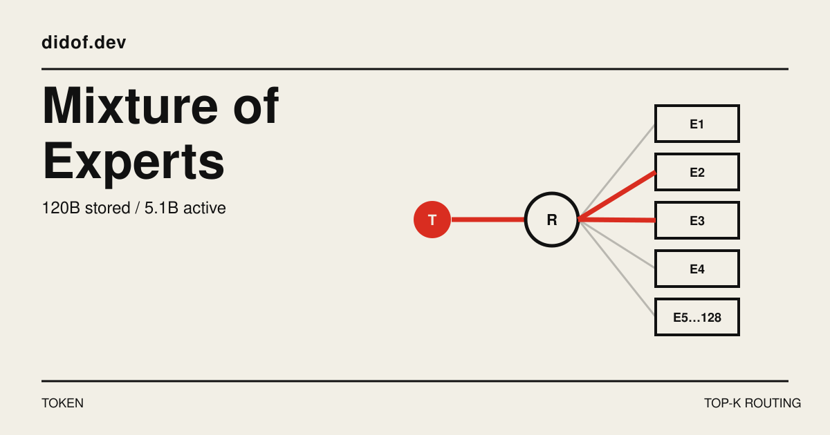
OpenAI’s gpt-oss-120b contains 116.8 billion parameters. For each token, it activates 5.1 billion.
That sounds like a contradiction. If the other 111.7 billion parameters are not doing the calculation, in what sense do they belong to the model?
The tempting explanation is that the model contains a panel of specialists. A router reads the question, recognizes that it is about mathematics or code, and sends the job to the right expert.
That is a useful first picture. It is also wrong in almost every detail.
The router does not usually assign the whole prompt to a specialist. It makes a new decision for each token, inside each Mixture of Experts, or MoE, layer. The “experts” are not small chatbots. They are alternative feed-forward networks: large sets of matrices that transform a token’s current internal representation.
This distinction explains both the efficiency and the hidden cost of Mixture of Experts. The architecture avoids many multiplications. It does not avoid storing, moving, and coordinating a very large model.
The part of a Transformer that gets duplicated
A Transformer block contains two major operations.
First, attention lets each token collect information from other tokens. This is where a word such as “bank” can acquire a different internal representation in “river bank” and “investment bank.”
Then a feed-forward network, or FFN, transforms each token representation independently. In simplified form:
Those linear transformations are large matrix multiplications. They also account for a substantial share of a language model’s parameters.
If that compact diagram hides the interesting part, the companion FFN walkthrough follows one contextualized token through expansion, activation, gating, contraction, and the residual path .
In a dense Transformer, every token passes through the same FFN at a given layer. A sparse Mixture-of-Experts model replaces that one FFN with several alternatives:
The model stores every expert, but a router selects only a small subset for each token. This is conditional computation: the parameters used by the calculation depend on the data currently passing through the network.
The modern sparsely gated version of this idea was demonstrated at large scale in the 2017 paper Outrageously Large Neural Networks . The core bargain has remained the same: increase parameter capacity much faster than computation per token.
Follow one token through the router
Suppose a layer contains eight experts and selects two of them for each token.
The router receives the token’s current hidden state, a vector we can call x. A learned linear projection converts that vector into one score per expert:
For one token, the output could look like this:
| Expert | Router score |
|---|---|
| E1 | 1.4 |
| E2 | -0.2 |
| E3 | 2.1 |
| E4 | 0.7 |
| E5–E8 | lower |
A Top-K operation keeps the highest K scores. With K = 2, only E3 and E1 survive. A normalization step turns their scores into weights. Imagine that it produces 0.67 for E3 and 0.33 for E1.
The layer computes:
The other six expert FFNs do not process this token.
Real models differ in the scoring and normalization details. gpt-oss, for example, selects the top four experts and applies softmax over those selected scores. OpenAI documents 128 experts per block in gpt-oss-120b, 32 in gpt-oss-20b, and Top-4 routing in both . DeepSeek-V3 computes token-to-expert affinities with a sigmoid, selects the highest values, then normalizes the selected affinities. Its technical report publishes the routing equations directly .
The variants matter to researchers and implementers. The stable idea is simpler: score every route, execute a few, combine their outputs.
The router does not route the question
The router sees a token representation, not a topic label.
That representation already contains context from the preceding attention operation. It can encode information about syntax, position, surrounding words, and patterns learned during training. The router uses that state to choose a path through this one layer.
At the next Mixture-of-Experts layer, the token has changed. A different router evaluates the new representation and can select a different pair of experts.
So one token can select E3 and E1 in layer 1, E7 and E2 in layer 2, then E2 and E5 in layer 3.
The next token can take another path through the same layers.
Mixtral 8×7B is a clean example. Each layer contains eight feed-forward experts. For every token, at every layer, the router selects two. The model has about 47 billion total parameters but uses about 13 billion active parameters during inference.
This is why “the coding expert answered the coding question” is the wrong model. There is no single handoff. There is a sequence of small routing decisions distributed across tokens and depth.
Why 120B does not become 120B divided by 32
gpt-oss-120b selects four experts out of 128. It would be easy to calculate:
But OpenAI reports 5.1 billion active parameters, not 3.75 billion.
The simple division fails because the entire model is not inside the expert pool. Attention, embeddings, output projections, normalization, routers, and other shared parts still run. Only the expert FFNs are sparsely activated.
OpenAI’s published breakdown makes the distinction visible:
| Component | Parameters in gpt-oss-120b |
|---|---|
| Expert multilayer perceptrons | 114.71B |
| Attention | 0.96B |
| Embedding and output | 1.16B |
| Total | 116.83B |
| Active per token | 5.13B |
“Active parameters” therefore describes a path through the model, not a smaller model hiding inside it.
There is another subtlety. The number is per token. During prompt processing or batched serving, many tokens are evaluated together. Each token may select only four experts, while the union of their choices can touch many more. With enough varied tokens in a batch, the hardware may need to execute work across most of the expert pool. Research on expert prefetching describes this growth from a single token’s K experts toward the full pool as batch size increases .
Sparse per-token computation does not imply that only four experts matter to the server at a time.
How the experts learn without assigned jobs
Nobody needs to label E17 as “Python” or E42 as “German grammar.” Router and experts are trained together with the rest of the model.
During a forward pass, the router selects a path. The selected expert outputs contribute to the model’s next-token prediction. When training measures the prediction error, backpropagation sends gradients through those expert computations and through the weights used to combine them.
That creates a feedback loop:
This is how specialization can emerge without a human taxonomy.
The hard Top-K boundary is not differentiable in the ordinary sense: an infinitesimal score change usually does not change which experts were selected. Training still obtains gradients through the selected gate weights, while MoE systems add routing-specific objectives or control mechanisms to keep the whole process useful.
That extra machinery is necessary because the same feedback loop can run away.
The best expert can become a traffic jam
Imagine that one expert performs slightly better early in training. The router sends it more tokens. Because it receives more tokens, it gets more updates. It improves faster, so the router sends it even more work.
Eventually, a few experts can absorb most of the traffic while the others barely train. This is commonly called routing collapse.
The problem is not only wasted model capacity. Experts are usually distributed across accelerators. If one GPU receives far more tokens than the others, the whole layer waits for that overloaded device.
Earlier architectures imposed a fixed capacity per expert. When too many tokens selected the same route, excess tokens could skip that expert computation and continue through the residual connection. Increasing the capacity reduced dropped tokens, but reserved more memory and computation for empty slots. Switch Transformer documents this trade-off and reports typical dropped-token rates below 1% in its experiments .
Switch Transformer also adds an auxiliary loss that encourages the router to distribute tokens across experts. This introduces a real tension:
- route by usefulness, and the same experts may become overloaded;
- route for perfect balance, and the model may avoid the expert it considers most useful.
DeepSeek-V3 uses a different control mechanism. Each routed expert has a bias that affects whether it enters the Top-K set. After a training step, the system lowers the bias of overloaded experts and raises the bias of underused ones. The original affinity score still determines how strongly a selected output contributes. DeepSeek also keeps a much smaller sequence-level balance loss to prevent extreme local imbalance.
The router is not optimizing in a mathematical vacuum. It is learning under the physical constraint that the work must fit across real machines.
What does an “expert” actually know?
The name encourages a tidy story: one expert learns science, another code, another French.
The evidence is less tidy.
Analyses of MoE models have found several kinds of routing patterns: token-level preferences, syntactic patterns, domain associations, repeated or overlapping expert behavior, and differences across layers and architectures. A 2024 analysis of Mixtral, DeepSeekMoE, and Grok found that Mixtral’s routing was relatively even and that instruction fine-tuning changed its routing patterns very little. The authors did not find one universal form of specialization. See A Closer Look into Mixture-of-Experts in Large Language Models .
A 2026 preprint that examined twelve MoE models argues for a more functional interpretation. Its experts were often associated with fine-grained linguistic or semantic operations, such as closing brackets in LaTeX, rather than broad subjects such as “mathematics.” The study did not include the largest models, including DeepSeek-V3, because of memory and compute limits.
The safe conclusion is not that experts lack specialization. It is that “expert” names a separately parameterized computational path, not a guaranteed human-readable profession.
The arithmetic gets cheaper. The logistics get harder
If a dense FFN has one set of parameters, making it wider usually increases both model capacity and the matrix multiplication performed for every token.
An MoE layer partially separates those quantities:
As long as K stays much smaller than N, the model can add parameter capacity without multiplying every token by every expert matrix.
That is the gain.
But an inactive expert is not an absent expert. Its weights must remain somewhere accessible because the next token, or the next layer, may select it.
The quantized gpt-oss-120b checkpoint is 60.8 GiB even though only 5.1 billion parameters are active per token. Quantization allows it to fit on one 80 GB accelerator, but the full expert pool still occupies memory.
If the pool does not fit on one accelerator, a serving system has two broad options.
It can distribute experts across several GPUs. Then each layer must send token representations to the devices that own the selected experts and retrieve the results. This dispatch-and-combine pattern creates all-to-all communication.
Or it can keep some experts in CPU memory or storage and load them on demand. That saves accelerator memory, but the router cannot know which weights are needed until it sees the current representation. Weight transfer can land directly on the latency-critical path. The same expert-prefetching study models this dependency explicitly and measures the cost of on-demand copies during decoding.
DeepSeek-V3 shows how serious the first problem becomes at scale. It has 256 routed experts per MoE layer, activates eight for each token, and distributes those experts across 64 GPUs. Its routing restricts each token to at most four nodes to reduce network traffic. The training system then overlaps communication with computation. The technical report describes separate attention, dispatch, expert computation, and combine phases .
The model saved multiplications and created a scheduling problem.
Why fewer active parameters do not guarantee lower latency
Parameter sparsity describes which mathematical operations are necessary. Wall-clock speed also depends on how efficiently the hardware performs them.
An MoE implementation can lose time by:
- moving token representations between devices;
- loading expert weights from slower memory;
- waiting for an overloaded expert;
- launching many small matrix operations that underuse the GPU;
- executing a wide set of experts across a large batch even though each token selects only a few.
On a large, carefully engineered cluster, those costs can be hidden or amortized. On a local machine constrained by memory bandwidth, they can dominate.
This is why “120B total, 5.1B active” is not a direct speed claim. It tells us something important about arithmetic. It does not tell us where the weights live, how many experts a batch touches, how far each token travels, or whether the runtime has efficient sparse kernels.
The distinction also explains why an MoE model can be cheaper to compute than a similarly capable dense model while remaining harder to deploy than its active-parameter count suggests.
The parameter count now describes two different things
For a dense model, total parameters and parameters used per token are nearly the same number. That made parameter count a rough, imperfect proxy for both capacity and computational cost.
Mixture of Experts breaks that shortcut.
The total parameter count describes how many learned weights the model can draw from. The active parameter count describes the route taken by one token. Neither describes inference by itself.
To understand the real cost, we need at least three quantities: total parameters, active parameters per token, and the hardware and communication required to keep every route available.
So the missing 111.7 billion parameters in gpt-oss-120b are not dormant decoration. They are alternative transformations waiting behind later routing decisions.
The model does not make 120 billion parameters cheap by pretending most of them do not exist. It makes their computation conditional, then pays to keep every possible path within reach.